Hybrid Transactional/Analytical Processing (HTAP)

It is common to divide data management environments in two classes, one being online transaction processing (OLTP), the other class is online analytical processing (OLAP). OLTP is characterized by large numbers of online transactions (create, replace, update, delete or CRUD operations). These transactions should happen very fast; applications running on top of a OLTP database often require instant responses. OLAP on the other hand is more concerned with historical data on which complex analytical processes need to run. The volumes of the transactions are much lower compared to OLTP, but the transactions are often very complex and involve larger amount of data. OLAP applications typically use machine learning techniques and the data are stored in a multi-dimensional schema or star schema.

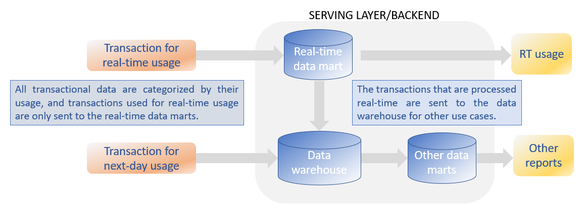
Because the same database instance is not able to support both activities with opposing demands, separate databases are setup, one database for OLTP, the other database supporting the analytical type of processes (OLAP). But the consequence of this segregation is that a constant dataflow needs to exist from the OLTP database to the OLAP database. This dataflow is called ETL (extract, transform and load). The ETL process will store the data from the OLTP database in another isolated environment such as a data warehouse or lately often in a data lake. Often a second ETL will move data from the data warehouse to another data store, called the data mart on which reports and ad-hoc queries are performed. Data warehouses rely on traditional RDBMS platforms, and the dimensional models in data marts are aligned to support the performance levels in accordance with the frequent and complex business analysis queries.

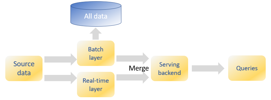
This process worked well until now because the reports were needed one day later. This time window was needed by the ETL process to move data from the source application to the data warehouses and the data marts. But lately there an increased demand for real-time reporting systems with the emergence of streaming data from sensors (IoT, internet of things), machine to machine data, social media and other operational data. On top of these new type of data, real-time analytics is required to provide recommendations to users and more personalized responses to any user interaction.

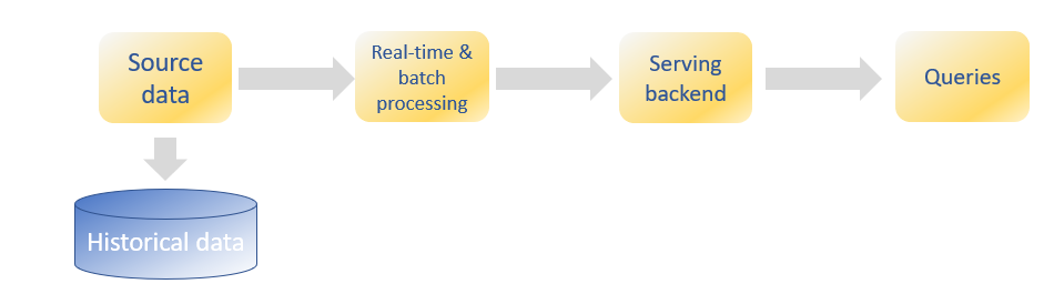
New database technologies have emerged the latest years that support hybrid workloads within one database instance. These new database systems take advantage of the new hardware technologies such as sold-state disks (SSD) and cost reductions in RAM memory. Gartner coined the term “Hybrid Transactional and Analytical Processing” (HTAP) to describe this new type of databases [3]. These database technologies allow for transactional and analytical processing to execute at the same time and on the same data [2]. Consequently, real-time processing and reports are possible at the same time that the transactions occur. Another term used to describe this type of processing is transactional analytics. The term indicates that insight and decision take place instantaneously with a transaction, e.g. at the moment of engagement with the customer, partner or device.

For example, a customer wants to buy a tablet in an online shop. During the selection process, the customer will get personalized recommendations in real time based on his previous and current surfing behavior. Once a tablet is put in the shopping basket and the payment transaction is initiated, fraud analytics is initiated in real time which is another transactional analytics process. In less than a minute all customer interactions are finalized with the aim to increase customer satisfaction and revenue. Note that these functions, fraud detection and recommendation systems exist today, but it requires a heterogenous and complex architecture. HTAP will simplify the architecture dramatically because all data are available in the same database and all analytical processes will occur in the same environment.

Traditional data architectures separate the transactions from the analytics which run on separate systems, each optimized for the particular type of processes and requirements. Data is copied from one system to the other one and those integration data pipelines will only add more complexity.

When we compare current architecture with a HTAP based architecture, the following differences are apparent:

  • Complex architecture. Current data architectures are complex because data is moved from the transactional systems to the analytical systems using ETL and other integration tools to move and transform the data. Also, enterprise service buses (ESB) are used to manage this complex architecture. These tools are not required anymore if transactional and analytical processes occur in the same system.
  • Real-time analytics. Because data is moved from the transactional to the analytical systems, a large time gap exists between the moment the transactions occurred and the moment these transactions can be analyzed.
  • Data duplication. Copying data from one system to the other system not only duplicates the data, but every complex ETL process might introduce data quality problems which leads to inconsistencies in the reporting.

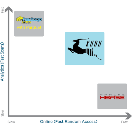
There are today several database implementations that use one or more HTAP features [1] such SAP HANA, MemSQL, IBM dashDB, Hyper, Apache Kudu, ArangoDB, Aerospike, etc.


[1] Hybrid Transactional/Analytical Processing: A Survey, Fatma Özcan et al. SIGMOD ’17, May 14–19, 2017, Chicago, IL, USA.

[2] Hybrid transactional/analytical processing (HTAP)  https://en.wikipedia.org/wiki/Hybrid_transactional/analytical_processing_(HTAP)

[3] Hybrid Transaction/Analytical Processing Will Foster Opportunities for Dramatic Business Innovation. Pezzini, Massimo et al.  Gartner. 28 January 2014

The real-time data mart and its integration in an enterprise data warehouse

It are challenging times; not only is there higher volumes on data to handle, and most predictions expect are an exponential increase, but more requests are received to have real-time or near real-time data. The value of real-time business data decreases when it gets older, but at the same time there is a higher demand on integrated and high-quality data which requires more processing power.

The main uses cases for real-time data marts are [2]:

  • Operational reporting and dashboards: Operational data that needs to be visualized for immediate actions using business intelligence tools.
  • Query offloading: replication of high-cost or legacy OLTP databases to another infrastructure of easy querying without impacts on the applications.
  • Real-time analytics: the data and the results of any predictive analytics process require often that actions are taken with the shortest delay possible, for example fraud detection.

There are large differences between the requirements for a real-time data mart and those for an enterprise data warehouse [6]. The following table lists some of the requirements of each data store:

  Real-time (RT) data mart Enterprise data warehouse (EDW)
Description Data is available in reports and dashboards from several source systems after a few seconds or a few minutes the latest. Data is available in reports and dashboards from ALL source systems next day or later. There are integrated and of high quality.
Latency Seconds/minutes Days/months
Capture Event-based/streaming Batch
Processing requirements Moderate High
Target loading impact Low impact High
User access/queries Yes No (used to feed the user access layer with data marts)

The techniques used vary mostly on the latency of data integration, from daily/monthly batches to streaming real-time integration. The capture of data from the application sources can be performed through queries that filter based on a timestamp or a flag, or through a change data capture (CDC) mechanism that detects any changes as it is happening. In case of streaming, the events are captured as they occur and are immediately integrated in the data mart. With a batch process, changes after a specified period are detected, rather than events. A daily batch mechanism is most suitable if intra-day freshness is not required for the data, such as longer-term trends or data that is only calculated once daily, for example financial close information. Batch loads might be performed in a downtime window, if the business model doesn’t require 24-hr availability of the data warehouse.

A well-known architecture to solve these conflicting requirements is the lambda architecture [3]. This architecture takes advantage of both batch- and stream-processing methods.

Lambda Architecture
Lambda Architecture

A more recent approach is the Kappa architecture [4], which removes the batch layer from the lambda architecture. It has many advantages, such as the need to write and maintain only code for the streaming layer. There are no two group of codes or frameworks; one for the batch and another for the streaming layer.

Kappa Architecture
Kappa Architecture

The kappa architecture treats a batch as a special case of a stream. A batch is a data set with a start and an end (bounded), while a stream has no start or end and is infinite (unbounded). Because a batch is a bounded stream, one can conclude that batch processing is a subset of stream processing.  Hence, the Lambda batch layer results can also be obtained by using a streaming engine. This simplification reduces the architecture to a single streaming engine capable of ingesting the needed volumes of data to handle both batch and real-time processing. Overall system complexity significantly decreases with Kappa architecture.

The streams (real-time and batch) are send to the serving back-end after processing. This serving back-end can contain the several components of a BI stack such as a data warehouse or a real-time data mart.

The BI architecture for the Serving Layer is shown in the next figure.

Serving Layer components

The transactions that are needed for real-time data marts are sent immediately to the data marts, while all other transactions (and referential data) are sent the data warehouse for long-term storage. The real-time transactions are sent in a second step to the data warehouse which makes that all data are present in the data warehouse. Note that this design pattern is also presented for the operational data store [1].

There will be many real-time data marts for a specific use case or business channel, but the data marts are should all use the same platform as the data warehouse and be integrated as described before. Else tactical/operational decision and strategic decision support will not be based on the same data which will lead to inconsistencies and poor execution. [5]

[1] Operational data store https://en.wikipedia.org/wiki/Operational_data_store

[2] Best Practices for Real-Time Data Warehousing  http://www.oracle.com/us/products/middleware/data-integration/realtime-data-warehousing-bp-2167237.pdf

[3] Lambda Architecture http://lambda-architecture.net/

[4] Understand Kappa Architecture in 2 minutes http://dataottam.com/2016/06/02/understand-kappa-architecture-in-2-minutes/

[5] Ten Mistakes to Avoid When Constructing a Real-Time Data Warehouse http://www.bi-bestpractices.com/view-articles/4766

[6] What is operational data store vs. data warehouse technology? http://searchdatamanagement.techtarget.com/answer/What-is-an-operational-data-store-vs-a-data-warehouse


Uses cases for Kudu

The big data landscape was until 1-3 years ago dominated by several storage systems, the first was Hadoop HDFS and later followed by Apache HBase, a NoSQL database. HDFS is great for high-speed writes and scans while the latter is well suited for random-access queries. A new storage engine, Apache Kudu tries to bridge the gap between those two uses cases.  Apache Kudu is a distributed, columnar database for structured, real-time data. Because Kudu has a schema, it is only suited for structured data, contrary to HBase which is schemaless. The data model resembles that of more traditional databases such as SybaseIQ or SAP Hana which uses columnar storage, that makes it well suited for OLAP queries. It is not an in-memory database such as SAP Hana, but uses persistent memory integrated in the block cache.

Because Apache Kudu allows both fast scan and random access, a big data architecture can be much simplified to address any analytics and business intelligence use case.  Kudu enables the use of the same storage engine for large scale batch jobs and complex data processing jobs that require fast random access and updates. As a result, applications that require both batch as well as real-time data processing capabilities can use Kudu for both types of workloads.

Another step in the data pipeline: from Kafka to Kudu

The data pipeline described in other post (link) gave an overview of the complete data flow from external api to visualization.

Streaming Data Pipeline

A Kafka consumer is created using the Python Client for Kafka and the python Kudu interfaces allows the data to be sent to a Kudu table.

The Kafka consumers is created using a consumer group id which allows offset management to be handled by Kafka.

from kafka import KafkaConsumer
import kudu
import json
import datetime

consumer = KafkaConsumer('aircheckr_city', bootstrap_servers='192.168.1.238:9092', group_id='test_kudu', auto_offset_reset='earliest')
while True:
    msg=next(consumer)

To be fault-tolerant, committing offsets is mandatory.

….
consumer.commit_async()

Before starting the infinite loop, a connection to the Kudu master is established:

client = kudu.connect(host='ubuntu243', port=7051)

When a message is read from the kafka topic, the records is send to Kudu (after transformation – not shown):

    table = client.table('impala::default.kudu_aircheckr_stream')
    session = client.new_session()
    op = table.new_insert(dictval)
    session.apply(op)
    try:
        session.flush()
    except kudu.KuduBadStatus as e:
        print("kudu bad status during flush")
        print(session.get_pending_errors())

Note the naming conventions for Kudu tables that are created via impala: impala::database_name.table_name.

Note that this is a solution for low volumes because the python script is executed on the node where the script is installed and not the complete cluster. If execution on the cluster is needed other solution such as spark streaming need to be considered.


Links

Python client for Apache Kafka: https://github.com/dpkp/kafka-python

Python interface for Apache Kudu: https://github.com/cloudera/kudu/tree/master/python

Using Kafka Consumer Groups: https://docs.confluent.io/current/clients/consumer.html

Kudu tables naming conventions: https://www.cloudera.com/documentation/enterprise/5-11-x/topics/impala_tables.html#kudu_tables

Sending data to Flume using Python

The pollution data are retrieved from an external api (see this post for more information) and send to Apache Flume. Apache Flume is a service for streaming data into Hadoop and other streaming applications. Apache Flume is a distributed, reliable, and available service for efficiently collecting, aggregating, and moving large amounts of streaming data.

For the streaming data pipeline on pollution in Flanders, the data was send to Hadoop HDFS and to Apache Kafka. A Flume source captures the data received from the external api.

The python code to send the data to the flume agent using json format. The standard JSONHandler needs a header and a body section. Also the headers of the request requires to specify the content type :

url_flume = 'http://<ip-address>:<port>'
payload = [{'headers': {}, 'body': data_clean }]
headers = {'content-type': 'application/json'}
response = requests.post(url_flume, data=json.dumps(payload), 
            headers=headers)

Every Flume agent has normally one source, a memory channel and a sink. The incoming data can however be sent to more than one sink. For each additional sink, the source needs another memory channel.
A flow multiplexer is defined that can replicate or selectively route an event to one or more channels.

The configuration of the agent to receive and send the data is given below.

# Name the components on this agent
aircheckr1.sources = http_aircheckr
aircheckr1.sinks = hdfs_sink kafka_sink
aircheckr1.channels = channel_hdfs channel_kafka

# Describe/configure the source
aircheckr1.sources.http_aircheckr.type = http
aircheckr1.sources.http_aircheckr.bind = 0.0.0.0
aircheckr1.sources.http_aircheckr.port = 9260

# Describe the sink
aircheckr1.sinks.hdfs_sink.type = hdfs
aircheckr1.sinks.hdfs_sink.hdfs.path = hdfs://192.168.1.242/flume/aircheckr
aircheckr1.sinks.hdfs_sink.hdfs.rollInterval = 86400
aircheckr1.sinks.hdfs_sink.hdfs.rollSize = 0

aircheckr1.sinks.kafka_sink.type = org.apache.flume.sink.kafka.KafkaSink
aircheckr1.sinks.kakfa_sink.kafka.bootstrap.servers = ubuntu238:9092
aircheckr1.sinks.kafka_sink.kafka.topic = aircheckr
aircheckr1.sinks.kafka_sink.flumeBatchSize = 10

# Use a channel which buffers events in memory
aircheckr1.channels.channel_hdfs.type = memory
aircheckr1.channels.channel_hdfs.capacity = 1000
aircheckr1.channels.channel_hdfs.transactionCapacity = 500

aircheckr1.channels.channel_kafka.type = memory
aircheckr1.channels.channel_kafka.capacity = 1000
aircheckr1.channels.channel_kafka.transactionCapacity = 10

# Bind the source and sinks to the channel
aircheckr1.sources.http_aircheckr.channels = channel_hdfs channel_kafka
aircheckr1.sinks.hdfs_sink.channel = channel_hdfs
aircheckr1.sinks.kafka_sink.channel = channel_kafka

Links:
Apache Flume: https://flume.apache.org/

Map of pollution in Flanders

The map (see live map here) shows the pollution on the level of the municipality for Flanders. The pollutants for which data are available are nitrogen dioxide (NO2), ozone (O3) and small particles (PM10/PM2.5). These data are retrieve from Aircheckr. An API is available to retrieve these open data, originally provided by the Belgian government.

Several (front-end) tools are used to visualize the data. The map on Flanders with municipalities is shown using jQuery with the plugin Mapael that is based on raphael.js. To retrieve the data from the database, an API was created using Python with Flask and Flask restful.

The schema given below shows the complete (near) real-time streaming data pipeline. The data are retrieved from the exteral API (aircheckr) and send to Apache Flume which stores the data in Hadoop for future batch processing and analytics and also to Apache Kafka. A consumer of Kafka is written in Python and the result is stored in Apache Kudu. At last an API makes the data available for visualization or further processing.

Streaming Data Pipeline

Links

Aircheckr:  http://www.aircheckr.com

Irceline: http://www.irceline.be/nl/documentatie/open-data

Mapael: https://www.vincentbroute.fr/mapael/

Raphael.js: http://dmitrybaranovskiy.github.io/raphael/

Flask: http://flask.pocoo.org/