Using Spark for Data Profiling or Exploratory Data Analysis

Data profiling is the process of examining the data available in an existing data source (e.g. a database or a file) and collecting statistics and information about that data. The purpose of these statistics may be to find out whether existing data can easily be used for other purposes. 

Before any dataset is used for advanced data analytics, an exploratory data analysis (EDA) or data profiling step is necessary. This is an ideal solution for datasets containing personal data because only aggregated data are shown. The Social-3 Personal Data Framework provides metadata and data profiling information of each available dataset. One of the earliest steps after the data ingestion step is the automated creation of a data profile.

Exploratory data analysis (EDA) or data profiling can help assess which data might be useful and reveals the yet unknown characteristics of such new dataset including data quality and data transformation requirements before data analytics can be used.

Data consumers can browse and get insight in the available datasets in the data lake of the Social-3 Personal Data Framework and can make informed decision on their usage and privacy requirements. The Social-3 Personal Data Framework contains a data catalogue that allows data consumers to select interesting datasets and put them in a “shopping basket” to indicate which datasets they want to use and how they want to use them.

Before using a dataset with any algorithm it is essential to understand how the data looks like and what are the edge cases and distribution of each attribute. Questions that need to be answered are related to the distribution of the attributes (columns of the table), the completeness or the missing data.

EDA can in a subsequent cleansing step be translated into constraints or rules that are then enforced. For instance, after discovering that the most frequent pattern for phone numbers is (ddd)ddd-dddd, this pattern can be promoted to the rule that all phone numbers must be formatted accordingly. Most cleansing tools can then either transform differently formatted numbers or at least mark them as violations.

Most of the EDA provides summary statistics for each attribute independently. However, some are based on pairs of attributes or multiple attributes. Data profiling should address following topics:

  • Completeness: How complete is the data? What percentage of records has missing or null values?
  • Uniqueness: How many unique values does an attribute have? Does an attribute that is supposed to be unique key, have all unique values?
  • Distribution: What is the distribution of values of an attribute?
  • Basic statistics: The mean, standard deviation, minimum, maximum for numerical attributes.
  • Pattern matching: What patterns are matched by data values of an attribute?
  • Outliers: Are there outliers in the numerical data?
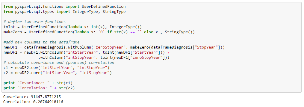
  • Correlation: What is the correlation between two given attributes? This kind of profiling may be important for feature analysis prior to building predictive models.
  • Functional dependency: Is there functional dependency between two attributes?

The advantages of EDA can be summarized as:

  • Find out what is in the data before using it
  • Get data quality metrics
  • Get an early assessment on the difficulties in creating business rules
  • Input the a subsequent cleansing step
  • Discover value patterns and distributions
  • Understanding data challenges early to avoid delays and cost overruns
  • Improve the ability to search the data

Data volumes can be so large that traditional EDA or data profiling, using for example a python script, for computing descriptive statistics become intractable. But even with scalable infrastructure like Hadoop, aggressive optimization and statistical approximation techniques must sometimes be used.

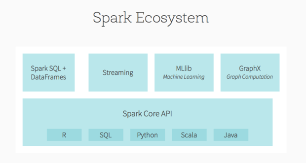
However, using Spark for data profiling or EDA might provide enough capabilities to compute summary statistics on very large datasets.

Exploratory data analysis or data profiling are typical steps performed using Python and R, but since Spark has introduced dataframes, it will be possible to do the exploratory data analysis step in Spark, especially for the larger datasets.

A DataFrame is a distributed collection of data organized into named columns. It is conceptually equivalent to a table in a relational database or a data frame in R/Python, but with richer optimizations under the hood. DataFrames can be constructed from a wide array of sources such as: structured data files, tables in Hive, external databases, or existing RDDs.

The data are stored in RDDs (with schema), which means you can also process the dataframes with the original RDD APIs, as well as algorithms and utilities in MLLib.

One of the useful functions for Spark Dataframes is the describe method. It returns summary statistics for numeric columns in the source dataframe. The summary statistics includes min, max, count, mean and standard deviations. It takes the names of one or more columns as arguments.

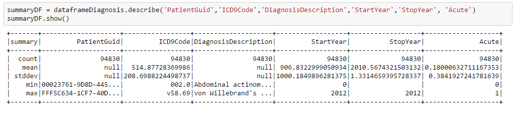
The above results provides information about missing data (e.g. a StartYear = 0, or an empty StopYear) and the type and range of data. Also notice that numeric calculations are sometimes made on a non-numeric field such as the ICD9Code.

The most basic form of data profiling is the analysis of individual columns in a given table. Typically, generated metadata comprises various counts, such as the number of values, the number of unique values, and the number of non-null values. Following statistics are calculated:

Statistics Description
Count Using the Dataframe describe method
Average Using the Dataframe describe method
Minimum Using the Dataframe describe method
Maximum Using the Dataframe describe method
Standard deviation Using the Dataframe describe method
Missing values Using the Dataframe filter method
Density Ratio calculation
Min. string length Using the Dataframe expr, groupBy, agg, min, max, avg methods
Max. string length Using the Dataframe expr, groupBy, agg, min, max, avg methods
# uniques values Using the Dataframe distinct and count methods
Top 100 of most frequent values Using the Dataframe groupBy, count, filter, orderBy, limit methods


This article was orginally posted at : http://www.social-3.com/solutions/personal_data_profiling.php


Hybrid Transactional/Analytical Processing (HTAP)

It is common to divide data management environments in two classes, one being online transaction processing (OLTP), the other class is online analytical processing (OLAP). OLTP is characterized by large numbers of online transactions (create, replace, update, delete or CRUD operations). These transactions should happen very fast; applications running on top of a OLTP database often require instant responses. OLAP on the other hand is more concerned with historical data on which complex analytical processes need to run. The volumes of the transactions are much lower compared to OLTP, but the transactions are often very complex and involve larger amount of data. OLAP applications typically use machine learning techniques and the data are stored in a multi-dimensional schema or star schema.

Because the same database instance is not able to support both activities with opposing demands, separate databases are setup, one database for OLTP, the other database supporting the analytical type of processes (OLAP). But the consequence of this segregation is that a constant dataflow needs to exist from the OLTP database to the OLAP database. This dataflow is called ETL (extract, transform and load). The ETL process will store the data from the OLTP database in another isolated environment such as a data warehouse or lately often in a data lake. Often a second ETL will move data from the data warehouse to another data store, called the data mart on which reports and ad-hoc queries are performed. Data warehouses rely on traditional RDBMS platforms, and the dimensional models in data marts are aligned to support the performance levels in accordance with the frequent and complex business analysis queries.

This process worked well until now because the reports were needed one day later. This time window was needed by the ETL process to move data from the source application to the data warehouses and the data marts. But lately there an increased demand for real-time reporting systems with the emergence of streaming data from sensors (IoT, internet of things), machine to machine data, social media and other operational data. On top of these new type of data, real-time analytics is required to provide recommendations to users and more personalized responses to any user interaction.

New database technologies have emerged the latest years that support hybrid workloads within one database instance. These new database systems take advantage of the new hardware technologies such as sold-state disks (SSD) and cost reductions in RAM memory. Gartner coined the term “Hybrid Transactional and Analytical Processing” (HTAP) to describe this new type of databases [3]. These database technologies allow for transactional and analytical processing to execute at the same time and on the same data [2]. Consequently, real-time processing and reports are possible at the same time that the transactions occur. Another term used to describe this type of processing is transactional analytics. The term indicates that insight and decision take place instantaneously with a transaction, e.g. at the moment of engagement with the customer, partner or device.

For example, a customer wants to buy a tablet in an online shop. During the selection process, the customer will get personalized recommendations in real time based on his previous and current surfing behavior. Once a tablet is put in the shopping basket and the payment transaction is initiated, fraud analytics is initiated in real time which is another transactional analytics process. In less than a minute all customer interactions are finalized with the aim to increase customer satisfaction and revenue. Note that these functions, fraud detection and recommendation systems exist today, but it requires a heterogenous and complex architecture. HTAP will simplify the architecture dramatically because all data are available in the same database and all analytical processes will occur in the same environment.

Traditional data architectures separate the transactions from the analytics which run on separate systems, each optimized for the particular type of processes and requirements. Data is copied from one system to the other one and those integration data pipelines will only add more complexity.

When we compare current architecture with a HTAP based architecture, the following differences are apparent:

  • Complex architecture. Current data architectures are complex because data is moved from the transactional systems to the analytical systems using ETL and other integration tools to move and transform the data. Also, enterprise service buses (ESB) are used to manage this complex architecture. These tools are not required anymore if transactional and analytical processes occur in the same system.
  • Real-time analytics. Because data is moved from the transactional to the analytical systems, a large time gap exists between the moment the transactions occurred and the moment these transactions can be analyzed.
  • Data duplication. Copying data from one system to the other system not only duplicates the data, but every complex ETL process might introduce data quality problems which leads to inconsistencies in the reporting.

There are today several database implementations that use one or more HTAP features [1] such SAP HANA, MemSQL, IBM dashDB, Hyper, Apache Kudu, ArangoDB, Aerospike, etc.


[1] Hybrid Transactional/Analytical Processing: A Survey, Fatma Özcan et al. SIGMOD ’17, May 14–19, 2017, Chicago, IL, USA.

[2] Hybrid transactional/analytical processing (HTAP)  https://en.wikipedia.org/wiki/Hybrid_transactional/analytical_processing_(HTAP)

[3] Hybrid Transaction/Analytical Processing Will Foster Opportunities for Dramatic Business Innovation. Pezzini, Massimo et al.  Gartner. 28 January 2014

Prediction of Traffic Speed using Spark and Kudu

The open data of traffic in Flanders contains not only data on traffic density, but also on the average speed per minute for 5 vehicle classes. In this blog post and the next blog posts, an attempt is made to create a predictive model for speed estimations (and not traffic density and traffic jams). Mainly during the night, one of the five vehicle classes (no. 2, cars) speeds above 120 km/h are often detected. A more detailed analysis of detected speed will be the subject for a next blog post, but most likely the results will not be different from those observed in The Netherlands. There are two limitations to these data: The speeds that are measured are an average speed during one minute and speeds above 250 km/h are not reliable.

I will start with the creation of a batch regression model based solely on the historical data on the average speed. In later iterations an attempt will be made to make more complex models such as:

    • include the information from previous time periods to make predictions about the current time period.
    • include weather information

The next chart shows average speed per hour for a specific measure point (Boomsesteenweg, Schelle).

Average Speed
Average Speed per hour

The data were retrieved using impala in a pyspark script:

from impala.dbapi import connect

conn = connect(host='kudu_master_ip', port=21050)
cur = conn.cursor()

uid = 2301
sqlStr = "select from_unixtime(cast(time as bigint), 'yyyy-MM-dd') as dy, dayofweek(time) as day_of_week, "
sqlStr+= " case when dayofweek(time) in (6,7) then 1 else 0 end as weekend_day, from_unixtime(cast(time as bigint), 'HH') as hr, "
sqlStr+= " avg(measure_class_2_speed) as avg_speed2, max(measure_class_2_speed) as max_speed2, "
sqlStr+= " from default.kudu_verkeer_stream "
sqlStr+= " where from_unixtime(cast(time as bigint), 'yyyy-MM-dd') >= '2017-01-01' and valid = 0 and uid = " + str(uid)
sqlStr+= " group by "
sqlStr+= " from_unixtime(cast(time as bigint), 'yyyy-MM-dd'), dayofweek(time), from_unixtime(cast(time as bigint), 'HH') "
cur.execute(sqlStr)
sqldata=cur.fetchall()

A simple feature selection is done:

datalist = []
for row in sqldata:
    datarow = [0,0,0,0,0,0,0,0,0,0,0,0,0,0,0,0,0,0,0,0,0,0,0,0,0,0,0]
    datarow[int(row[3])] = 1
    datarow[24] = row[1]
    datarow[25] = row[2]
    datarow[26] = int(row[3])
    datalist.append(LabeledPoint(row[4], datarow))

data=sc.parallelize(datalist)

Next a regression model is created using Spark MLLib.  The Spark ecosystem contains several modules including a library for machine learning, MLLib, graph computations (via GraphX), streaming (real-time calculations), and real-time interactive query processing with Spark SQL and DataFrames.

Most modules have a Python API.  Here I have used the regression algorithms module. A predictive model was created using Ridge regression.

from pyspark.mllib.regression import LabeledPoint, RidgeRegressionWithSGD

lrm = RidgeRegressionWithSGD.train(data, iterations=500, step=0.025, intercept=True, regParam=0.005)

The weights for each feature are:

Weights Value
intercept 4.36571
0h 0.63734
1h 0.10966
2h -0.21648
3h -0.23896
4h 0.15326
5h 0.48998
6h 0.58346
7h 0.76605
8h 0.62572
9h 0.49076
10h 0.42505
11h 0.41065
12h 0.30644
13h 0.21880
14h 0.10592
15h 0.07667
16h 0.02955
17h 0.00451
18h 0.04812
19h 0.01284
20h -0.00428
21h -0.27189
22h -0.48977
23h -0.90398
dow 4.61585
weekend -0.70381
hr 2.52832

I have not created a training, test or validation set here, but I still want to show the result of the prediction (so most likely overfitted):


The same behavior is seen for other measure points (E40, Kortenberg).

Note than this predictive model indicates that the average speed increases during the week, with the lowest average speed on Monday and a steady increase until Sunday.

When the average (and maximum) speed is calculated per day of the week, this trend is clear for the observed data. The chart below shows the speed for a measure point on the E40 at Kortenberg.  The average speed is low on Monday (70 km/h), but gradually increases the next days with the highest average speed recorded on Sunday (95 km/h). The maximum speed does not change that much: 139 km/h during all days, expect Sunday where a slight increase is recorded (143 km/h). However, this might be an artifact of the measurement method, because the average speed per minute is provided which might increase the maximum speed when the traffic density is low.

A second trend is the increase in average and maximum speed during the night


Flume monitoring

The Flume agents can be monitored individually by adding two parameters:

flume-ng agent -n agent_name -c conf -f conf config.conf -Dflume.monitoring.type=http -Dflume.monitoring.port=19256

The parameters flume.monitoring.type=http and flume.monitoring.port=24105 enable JSON monitoring.

The metrics are retrieved with following URL: http://<ip-address-agent:24105/metrics

Example of a response:

{
    "SOURCE.http_traffic":{"OpenConnectionCount":"0","Type":"SOURCE","AppendBatchAcceptedCount":"2561700","AppendBatchReceivedCount":"2561700","EventAcceptedCount":"2561700","AppendReceivedCount":"0","StopTime":"0","StartTime":"1504012941615","EventReceivedCount":"2561700","AppendAcceptedCount":"0"},
    "SINK.k4":{"Type":"SINK","ConnectionClosedCount":"0","EventDrainSuccessCount":"2561700","KafkaEventSendTimer":"17461960","ConnectionFailedCount":"0","BatchCompleteCount":"0","EventDrainAttemptCount":"0","ConnectionCreatedCount":"0","BatchEmptyCount":"679409","StopTime":"0","RollbackCount":"0","StartTime":"1504012941570","BatchUnderflowCount":"3942"},
    "CHANNEL.c4":{"EventPutSuccessCount":"2561700","ChannelFillPercentage":"0.0","Type":"CHANNEL","StopTime":"0","EventPutAttemptCount":"2561700","ChannelSize":"0","StartTime":"1504012941382","EventTakeSuccessCount":"2561700","ChannelCapacity":"5000","EventTakeAttemptCount":"3245052"},
    "CHANNEL.c1":{"EventPutSuccessCount":"2561700","ChannelFillPercentage":"0.0","Type":"CHANNEL","StopTime":"0","EventPutAttemptCount":"2561700","ChannelSize":"0","StartTime":"1504012941382","EventTakeSuccessCount":"2561700","ChannelCapacity":"5000","EventTakeAttemptCount":"3242098"},
    "CHANNEL.c3":{"EventPutSuccessCount":"2561700","ChannelFillPercentage":"0.0","Type":"CHANNEL","StopTime":"0","EventPutAttemptCount":"2561700","ChannelSize":"0","StartTime":"1504012941381","EventTakeSuccessCount":"2561700","ChannelCapacity":"5000","EventTakeAttemptCount":"3245036"},
    "SINK.k3":{"BatchCompleteCount":"22260","ConnectionFailedCount":"15","EventDrainAttemptCount":"2561701","ConnectionCreatedCount":"2228","Type":"SINK","BatchEmptyCount":"679389","ConnectionClosedCount":"2223","EventDrainSuccessCount":"2561700","StopTime":"0","StartTime":"1504012941383","BatchUnderflowCount":"3942"}
}

The source metrics are listen in the next table.

Table: Source metrics
Metric Description
EventReceivedCount The total number of events that the source has received until now.
EventAcceptedCount The total number of events where the event was successfully written out to the channel and the source returned success to the sink/RPC client/system that created the event.
AppendReceivedCount The total number of events that came in with only one event per batch (the equivalent of an append call in RPC calls).
AppendAcceptedCount The total number of events that came in individually that were written to the channel and returned successfully.
AppendBatchReceivedCount The total number of batches of events received.
AppendBatchAcceptedCount The total number of batches successfully committed to the channel.
StartTime Milliseconds since the epoch when the source was started.
StopTime Milliseconds since the epoch when the source was stopped.
OpenConnectionCount The number of connections currently open with clients/sinks (only an Avro Source currently exposes this). Type For sources, this always returns SOURCE.

The next table gives more information on the channel metrics.

Table: Channel metrics
Metric Description
ChannelSize The total number of events currently in the channel.
EventPutAttemptCount The total number of events the source(s) attempted to write to the channel.
EventPutSuccessCount The total number of events that were successfully written and committed to the channel.
EventTakeAttemptCount The total number of times the sink(s) attempted to read events from the channel. This does not mean that events were returned each time, since sinks might poll and the channel might not have any data.
EventTakeSuccessCount The total number of events that were successfully taken by the sink(s).
StartTime Milliseconds since the epoch when the channel was started.
StopTime Milliseconds since the epoch when the channel was stopped.
ChannelCapacity The capacity of the channel.
ChannelFillPercentage The percentage of the channel that is full. Type For channels, this always returns CHANNEL.

The Sink metrics given are:

Table: Sink metrics
Metric Description
ConnectionCreatedCount The number of connections created with the next hop or storage system (like when a new file is created on HDFS).
ConnectionClosedCount The number of connections closed with the next hop or storage system (like when a file on HDFS is closed).
ConnectionFailedCount The number of connections that were closed due to an error with the next hop or storage system (like when a new file on HDFS is closed because of timeouts).
BatchEmptyCount The number of batches that were empty—a high number indicates that the sources are writing data slower than the sinks are clearing it.
BatchUnderflowCount The number of batches that were smaller than the maximum batch size this sink is configured to use—this also indicates sinks are faster than sources if it’s high.
BatchCompleteCount The number of batches that were equal to the maximum batch size.
EventDrainAttemptCount The total number of events the sink tried to write out to storage.
EventDrainSuccessCount The total number of events that the sink successfully wrote out to storage.
StartTime Milliseconds since the epoch when the sink was started.
StopTime Milliseconds since the epoch when the sink was stopped. Type For sinks, this always returns SINK.

Note that Flume monitoring is also available with Cloudera Manager or Hortonworks Ganglia.

The real-time data mart and its integration in an enterprise data warehouse

It are challenging times; not only is there higher volumes on data to handle, and most predictions expect are an exponential increase, but more requests are received to have real-time or near real-time data. The value of real-time business data decreases when it gets older, but at the same time there is a higher demand on integrated and high-quality data which requires more processing power.

The main uses cases for real-time data marts are [2]:

  • Operational reporting and dashboards: Operational data that needs to be visualized for immediate actions using business intelligence tools.
  • Query offloading: replication of high-cost or legacy OLTP databases to another infrastructure of easy querying without impacts on the applications.
  • Real-time analytics: the data and the results of any predictive analytics process require often that actions are taken with the shortest delay possible, for example fraud detection.

There are large differences between the requirements for a real-time data mart and those for an enterprise data warehouse [6]. The following table lists some of the requirements of each data store:

  Real-time (RT) data mart Enterprise data warehouse (EDW)
Description Data is available in reports and dashboards from several source systems after a few seconds or a few minutes the latest. Data is available in reports and dashboards from ALL source systems next day or later. There are integrated and of high quality.
Latency Seconds/minutes Days/months
Capture Event-based/streaming Batch
Processing requirements Moderate High
Target loading impact Low impact High
User access/queries Yes No (used to feed the user access layer with data marts)

The techniques used vary mostly on the latency of data integration, from daily/monthly batches to streaming real-time integration. The capture of data from the application sources can be performed through queries that filter based on a timestamp or a flag, or through a change data capture (CDC) mechanism that detects any changes as it is happening. In case of streaming, the events are captured as they occur and are immediately integrated in the data mart. With a batch process, changes after a specified period are detected, rather than events. A daily batch mechanism is most suitable if intra-day freshness is not required for the data, such as longer-term trends or data that is only calculated once daily, for example financial close information. Batch loads might be performed in a downtime window, if the business model doesn’t require 24-hr availability of the data warehouse.

A well-known architecture to solve these conflicting requirements is the lambda architecture [3]. This architecture takes advantage of both batch- and stream-processing methods.

Lambda Architecture
Lambda Architecture

A more recent approach is the Kappa architecture [4], which removes the batch layer from the lambda architecture. It has many advantages, such as the need to write and maintain only code for the streaming layer. There are no two group of codes or frameworks; one for the batch and another for the streaming layer.

Kappa Architecture
Kappa Architecture

The kappa architecture treats a batch as a special case of a stream. A batch is a data set with a start and an end (bounded), while a stream has no start or end and is infinite (unbounded). Because a batch is a bounded stream, one can conclude that batch processing is a subset of stream processing.  Hence, the Lambda batch layer results can also be obtained by using a streaming engine. This simplification reduces the architecture to a single streaming engine capable of ingesting the needed volumes of data to handle both batch and real-time processing. Overall system complexity significantly decreases with Kappa architecture.

The streams (real-time and batch) are send to the serving back-end after processing. This serving back-end can contain the several components of a BI stack such as a data warehouse or a real-time data mart.

The BI architecture for the Serving Layer is shown in the next figure.

Serving Layer components

The transactions that are needed for real-time data marts are sent immediately to the data marts, while all other transactions (and referential data) are sent the data warehouse for long-term storage. The real-time transactions are sent in a second step to the data warehouse which makes that all data are present in the data warehouse. Note that this design pattern is also presented for the operational data store [1].

There will be many real-time data marts for a specific use case or business channel, but the data marts are should all use the same platform as the data warehouse and be integrated as described before. Else tactical/operational decision and strategic decision support will not be based on the same data which will lead to inconsistencies and poor execution. [5]

[1] Operational data store https://en.wikipedia.org/wiki/Operational_data_store

[2] Best Practices for Real-Time Data Warehousing  http://www.oracle.com/us/products/middleware/data-integration/realtime-data-warehousing-bp-2167237.pdf

[3] Lambda Architecture http://lambda-architecture.net/

[4] Understand Kappa Architecture in 2 minutes http://dataottam.com/2016/06/02/understand-kappa-architecture-in-2-minutes/

[5] Ten Mistakes to Avoid When Constructing a Real-Time Data Warehouse http://www.bi-bestpractices.com/view-articles/4766

[6] What is operational data store vs. data warehouse technology? http://searchdatamanagement.techtarget.com/answer/What-is-an-operational-data-store-vs-a-data-warehouse


Real-time traffic data

The Roads and Traffic Agency (Agentschap Wegen en Verkeer) [2] and the Flemish Traffic Centre (Vlaams Verkeerscentrum) [3] provide open data about the current traffic situation [1]. More of 4000 measurement points dispersed all over Flanders – but mainly located on highways, detect each minute the number of vehicles and their speed.

We use the same front-end and data pipeline as presented for the pollution data [4]. Because the amount of data is pretty big (more than 4000 measurements each minute), only a small selection of measurement points (~ 100) is captured every 10 minutes by an edge node and send to flume for further processing [5]. Two streams are captured, one with the list of measurement points and the second with the real-time traffic data (see figure).

Real Time Traffic Data Pipeline

The traffic data are send to Apache Kafka [6] and two topics are created. The topic with measurement points are stored in Apache Hive [7] to have a structured query interface for further processing. The topic with the real-time traffic data is consumed with a python script and enriched with the measurement points stored in Hive to create a new Kafka topic with the enriched traffic data (see figure). This new topic is read by Druid [8] for visualization and data discovery using several tools such as Apache Superset [9].

The two other Kafka topics are send to Kudu tables which are used for the visualizations (see live map here).


[1] Meten-in-Vlaanderen (MIV) http://opendata.vlaanderen.be/dataset/minuutwaarden-verkeersmetingen-vlaanderen

[2] Agentschap Wegen en Verkeer http://www.wegenenverkeer.be/

[3] Vlaams Verkeerscentrum http://www.verkeerscentrum.be/

[4] Map of pollution in Flanders http://www.bigdatareflections.net/blog/?p=1

[5] Sending data to Flume using Python http://www.bigdatareflections.net/blog/?p=35

[6] Apache Kafka https://kafka.apache.org/

[7] Apache Hive https://hive.apache.org/

[8] Druid http://druid.io/

[9] Using Superset with Kudu http://www.bigdatareflections.net/blog/?p=52


Using Superset with Kudu

Apache Superset is a visualization tool, originally developed by Airbnb [1]. The goal to develop this tool is to empower every user of data, especially users for which SQL is often a too high barrier. A second goal is to allow users to explore and discover insights with a user-friendly interface. The solution to both of these challenges is the development of Superset. Only recently it became an Apache project [2].

Once Apache superset is running, a new database connection is made using Impala. The URI has the format impala://<host>:21050/<database>.

Note that first the impala driver needs to be installed (pip install impyla) [3]

Next, a table is created to enable the usage of a dataset inside a slice or dashboard. Because only one data source can be used for each slice, the tables will often be a view of several tables that are joined beforehand. [4] This means if your tables are designed as dimensions and facts, a join between all tables needs to be made when the “table” is defined, or else a single table needs to be materialized that contain all table in the data source.

Once that table/view is defined, columns and metrics need to be defined before it can be used to define a slice.

At last, the slice can be created and added to a dashboard.

Links

[1] Superset: Scaling Data Access and Visual Insights at Airbnb  https://medium.com/airbnb-engineering/superset-scaling-data-access-and-visual-insights-at-airbnb-3ce3e9b88a7f

[2] Apache Superset (incubating) https://superset.incubator.apache.org/

[3] Installation & Configuration http://superset.apache.org/installation.html

[4] FAQ http://superset.apache.org/faq.html


Uses cases for Kudu

The big data landscape was until 1-3 years ago dominated by several storage systems, the first was Hadoop HDFS and later followed by Apache HBase, a NoSQL database. HDFS is great for high-speed writes and scans while the latter is well suited for random-access queries. A new storage engine, Apache Kudu tries to bridge the gap between those two uses cases.  Apache Kudu is a distributed, columnar database for structured, real-time data. Because Kudu has a schema, it is only suited for structured data, contrary to HBase which is schemaless. The data model resembles that of more traditional databases such as SybaseIQ or SAP Hana which uses columnar storage, that makes it well suited for OLAP queries. It is not an in-memory database such as SAP Hana, but uses persistent memory integrated in the block cache.

Because Apache Kudu allows both fast scan and random access, a big data architecture can be much simplified to address any analytics and business intelligence use case.  Kudu enables the use of the same storage engine for large scale batch jobs and complex data processing jobs that require fast random access and updates. As a result, applications that require both batch as well as real-time data processing capabilities can use Kudu for both types of workloads.

Another step in the data pipeline: from Kafka to Kudu

The data pipeline described in other post (link) gave an overview of the complete data flow from external api to visualization.

Streaming Data Pipeline

A Kafka consumer is created using the Python Client for Kafka and the python Kudu interfaces allows the data to be sent to a Kudu table.

The Kafka consumers is created using a consumer group id which allows offset management to be handled by Kafka.

from kafka import KafkaConsumer
import kudu
import json
import datetime

consumer = KafkaConsumer('aircheckr_city', bootstrap_servers='192.168.1.238:9092', group_id='test_kudu', auto_offset_reset='earliest')
while True:
    msg=next(consumer)

To be fault-tolerant, committing offsets is mandatory.

….
consumer.commit_async()

Before starting the infinite loop, a connection to the Kudu master is established:

client = kudu.connect(host='ubuntu243', port=7051)

When a message is read from the kafka topic, the records is send to Kudu (after transformation – not shown):

    table = client.table('impala::default.kudu_aircheckr_stream')
    session = client.new_session()
    op = table.new_insert(dictval)
    session.apply(op)
    try:
        session.flush()
    except kudu.KuduBadStatus as e:
        print("kudu bad status during flush")
        print(session.get_pending_errors())

Note the naming conventions for Kudu tables that are created via impala: impala::database_name.table_name.

Note that this is a solution for low volumes because the python script is executed on the node where the script is installed and not the complete cluster. If execution on the cluster is needed other solution such as spark streaming need to be considered.


Links

Python client for Apache Kafka: https://github.com/dpkp/kafka-python

Python interface for Apache Kudu: https://github.com/cloudera/kudu/tree/master/python

Using Kafka Consumer Groups: https://docs.confluent.io/current/clients/consumer.html

Kudu tables naming conventions: https://www.cloudera.com/documentation/enterprise/5-11-x/topics/impala_tables.html#kudu_tables

Sending data to Flume using Python

The pollution data are retrieved from an external api (see this post for more information) and send to Apache Flume. Apache Flume is a service for streaming data into Hadoop and other streaming applications. Apache Flume is a distributed, reliable, and available service for efficiently collecting, aggregating, and moving large amounts of streaming data.

For the streaming data pipeline on pollution in Flanders, the data was send to Hadoop HDFS and to Apache Kafka. A Flume source captures the data received from the external api.

The python code to send the data to the flume agent using json format. The standard JSONHandler needs a header and a body section. Also the headers of the request requires to specify the content type :

url_flume = 'http://<ip-address>:<port>'
payload = [{'headers': {}, 'body': data_clean }]
headers = {'content-type': 'application/json'}
response = requests.post(url_flume, data=json.dumps(payload), 
            headers=headers)

Every Flume agent has normally one source, a memory channel and a sink. The incoming data can however be sent to more than one sink. For each additional sink, the source needs another memory channel.
A flow multiplexer is defined that can replicate or selectively route an event to one or more channels.

The configuration of the agent to receive and send the data is given below.

# Name the components on this agent
aircheckr1.sources = http_aircheckr
aircheckr1.sinks = hdfs_sink kafka_sink
aircheckr1.channels = channel_hdfs channel_kafka

# Describe/configure the source
aircheckr1.sources.http_aircheckr.type = http
aircheckr1.sources.http_aircheckr.bind = 0.0.0.0
aircheckr1.sources.http_aircheckr.port = 9260

# Describe the sink
aircheckr1.sinks.hdfs_sink.type = hdfs
aircheckr1.sinks.hdfs_sink.hdfs.path = hdfs://192.168.1.242/flume/aircheckr
aircheckr1.sinks.hdfs_sink.hdfs.rollInterval = 86400
aircheckr1.sinks.hdfs_sink.hdfs.rollSize = 0

aircheckr1.sinks.kafka_sink.type = org.apache.flume.sink.kafka.KafkaSink
aircheckr1.sinks.kakfa_sink.kafka.bootstrap.servers = ubuntu238:9092
aircheckr1.sinks.kafka_sink.kafka.topic = aircheckr
aircheckr1.sinks.kafka_sink.flumeBatchSize = 10

# Use a channel which buffers events in memory
aircheckr1.channels.channel_hdfs.type = memory
aircheckr1.channels.channel_hdfs.capacity = 1000
aircheckr1.channels.channel_hdfs.transactionCapacity = 500

aircheckr1.channels.channel_kafka.type = memory
aircheckr1.channels.channel_kafka.capacity = 1000
aircheckr1.channels.channel_kafka.transactionCapacity = 10

# Bind the source and sinks to the channel
aircheckr1.sources.http_aircheckr.channels = channel_hdfs channel_kafka
aircheckr1.sinks.hdfs_sink.channel = channel_hdfs
aircheckr1.sinks.kafka_sink.channel = channel_kafka

Links:
Apache Flume: https://flume.apache.org/